FM Theory
Simple FM: one carrier, one modulator
The basic mathematical function for simple FM looks surprisingly simple:
\[y = sin(x+sin(x))\]
In this formula, a sine wave is modulated with another sinewave with the same frequency. Let:
- \(F_c\) the frequency of the carrier;
- \(F_m\) the frequency of the modulator;
- \(C\) the frequency-ratio of the carrier (we will mostly use \(C=1\));
- \(M\) the frequency-ratio of the modulator;
- \(I\) the modulation index: the amount of modulation;
- \(k=0,1,2,3,..\) the sideband order \(k\)
Using \(C\), \(M\) and \(I\) in the original formula, we get:
\[y = sin(Cx+I*sin(Mx))\]
To compute the actual frequency spectrum, we need to consider the sidebands from the original carrier frequency \(F_c\). The 0th order sideband is the frequency \(F_c\). Sideband orders range from \(k=0,1,2,3,..\) Both left sidebands (frequencies to the left of the carrier frequency) and right sidebands (frequencies to the right of the carrier frequency) occur. The actual frequencies of such a sideband is related to the modulation frequency:
\[F_c ± k*F_m\]
You only have to compute the \(I+2\) order sideband, all other sidebands will have a negible amplitudes.
The amplitude of a particular order sideband \(k\) is calculated using the Bessel function of the same order \(k\) of the modulation index \(I\):
\[Amplitude = J_k(I)\]
A sideband corresponds to a frequency, so we get the amplitude of the sine wave for that frequency. But we have some things to consider:
- A sideband at frequency 0Hz is actually a DC offset, so if such a sideband would occur we can ignore this sideband.
- Bessel functions with order above 3 can have negative results, so the calculated amplitude is actually negative.
- Odd sidebands to the left of the original frequency have a phase shift of 180 degrees. As such a phase shift for a sine wave corresponds to a negative amplitude of the original phase, this can be represented by a sign change of the amplitude. The same result can be found by using negative orders for the Bessel function: \(J_{-k}(I) = -J_k(I))\text{ for odd n}\).
- A wave with a negative frequency is actually a wave with the same positive frequency, but with a phase shift of 180 degrees: if you would “plot” a negative frequency: the sine wave would go “back” along the x axis, which looks like the same sine wave going forward along the x-axis, but with just a phase shift of 180 degrees. And such a phase shift is simply a sign change of the amplitude. This means that we can consider a sideband with a negative frequency as a sideband with the same positive frequency, but with a sign-change of the amplitude (positive becomes negative, negative becomes positive).
Feedback
Feedback is the result of feeding the output of the oscillator back into itself:
\[y = sin(x + I * sin(y))]\]
The feedback function resembles the original modulation formula. With feedback, only positive sidebands will occur. The amplitude of each sideband is calculated using the following formula:
\[Amplitude = 2 * \dfrac{J_k(I * k)}{I * k}\]
This function won’t work for I = 0 (division by zero), but interestingly, the whole function resolved to 0 for k>1 and to 1 for k=1 (as you would expect: just a regular sinoid wave at feedback level zero).
Unlike “plain” FM, with feedback, the higher sidebands do really add up: you need to calculate a lot of them. From around modulation index 1.3, negative frequencies occur at the highest feedback levels. This introduces noise in the calculated FM wave, but not in the sidebands: they still add up nicely (although resulting in a wave with an increasingly lower amplitude).
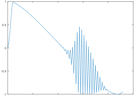
The burst of noise is actually the oscillator going very rapidly going between two extreme values, that’s why two separate lines are visible. Using Octave, we can plot the graph above that depicts what is going on (see feedback.m for the script).
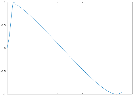
The noise burst is the result of the sampling rate of digital synthesizers. It is the reason that Yamaha originally used an averaging filter for the feedback, using not only the previous value, but actually the average between the previous two values, which will make the noise burst disappear. The explanation is mentioned in this patent, as is visible in the graph below, using the same parameters, but with the average filter (see feedback-filter.m for the script).
Interestingly the “pure” math equation results in a graph that is actually “not possible” from a sound perspective (it goes “back in time”):
\(y = sin(x + 1.4 * sin(y))\) (show math)